The new ggseg-package version has introduced a new way of plotting
the brain atlases, through a custom geom_brain (variant of
geom_sf). This has introduced a lot of new functionality into the
package, in addition to some new custom methods and objects.
The brain-atlas class
The first new thing to notice is that we have introduced a new atlas
class called brain-atlas. This class is a special class for
ggseg-atlases, that contain information in a specific way. They are
objects with 4-levels, each containing important information about the
atlas in question.
library(ggseg)
dk$atlas
#> [1] "dk"
dk$type
#> [1] "cortical"
dk$palette
#>                   bankssts  caudal anterior cingulate
#>                  "#196428"                  "#7D64A0"
#>      caudal middle frontal            corpus callosum
#>                  "#641900"                  "#784632"
#>                     cuneus                 entorhinal
#>                  "#DC1464"                  "#DC140A"
#>                   fusiform          inferior parietal
#>                  "#B4DC8C"                  "#DC3CDC"
#>          inferior temporal          isthmus cingulate
#>                  "#B42878"                  "#8C148C"
#>          lateral occipital      lateral orbitofrontal
#>                  "#141E8C"                  "#234B32"
#>                    lingual       medial orbitofrontal
#>                  "#E18C8C"                  "#C8234B"
#>            middle temporal            parahippocampal
#>                  "#A06432"                  "#14DC3C"
#>                paracentral           pars opercularis
#>                  "#3CDC3C"                  "#DCB48C"
#>             pars orbitalis          pars triangularis
#>                  "#146432"                  "#DC3C14"
#>              pericalcarine                postcentral
#>                  "#78643C"                  "#DC1414"
#>        posterior cingulate                 precentral
#>                  "#DCB4DC"                  "#3C14DC"
#>                  precuneus rostral anterior cingulate
#>                  "#A08CB4"                  "#50148C"
#>     rostral middle frontal           superior frontal
#>                  "#4B327D"                  "#14DCA0"
#>          superior parietal          superior temporal
#>                  "#14B48C"                  "#8CDCDC"
#>              supramarginal               frontal pole
#>                  "#50A014"                  "#640064"
#>              temporal pole        transverse temporal
#>                  "#464646"                  "#9696C8"
#>                     insula
#>                  "#FFC020"
dk$data
#> Simple feature collection with 90 features and 5 fields
#> Geometry type: MULTIPOLYGON
#> Dimension:     XY
#> Bounding box:  xmin: 0 ymin: 0 xmax: 1390.585 ymax: 205.4407
#> CRS:           NA
#> # A tibble: 90 × 6
#>    hemi  side    region                label     roi                    geometry
#>  * <chr> <chr>   <chr>                 <chr>     <chr>            <MULTIPOLYGON>
#>  1 left  lateral NA                    NA        0001  (((84.32563 34.46407, 84…
#>  2 left  lateral bankssts              lh_banks… 0002  (((214.8215 108.8139, 21…
#>  3 left  lateral caudal middle frontal lh_cauda… 0004  (((106.16 184.3144, 93.6…
#>  4 left  lateral fusiform              lh_fusif… 0008  (((256.5481 48.35713, 24…
#>  5 left  lateral inferior parietal     lh_infer… 0009  (((218.4373 161.6233, 21…
#>  6 left  lateral inferior temporal     lh_infer… 0010  (((250.7745 70.75764, 24…
#>  7 left  lateral lateral occipital     lh_later… 0012  (((277.4615 115.0523, 27…
#>  8 left  lateral lateral orbitofrontal lh_later… 0013  (((66.26648 69.56474, 56…
#>  9 left  lateral middle temporal       lh_middl… 0016  (((238.0128 91.25816, 23…
#> 10 left  lateral pars opercularis      lh_parso… 0019  (((79.03391 126.496, 74.…
#> # ℹ 80 more rows
Of these four, only the palette is an optional part,
where some atlases may have this field empty. The data, you might
notice, is simple-features data, with a geometry column
that includes all the information needed to plot the data as a simple
features object. You can actually call plot directly on the
data, and the standard simple features plot will appear.
plot(dk$data)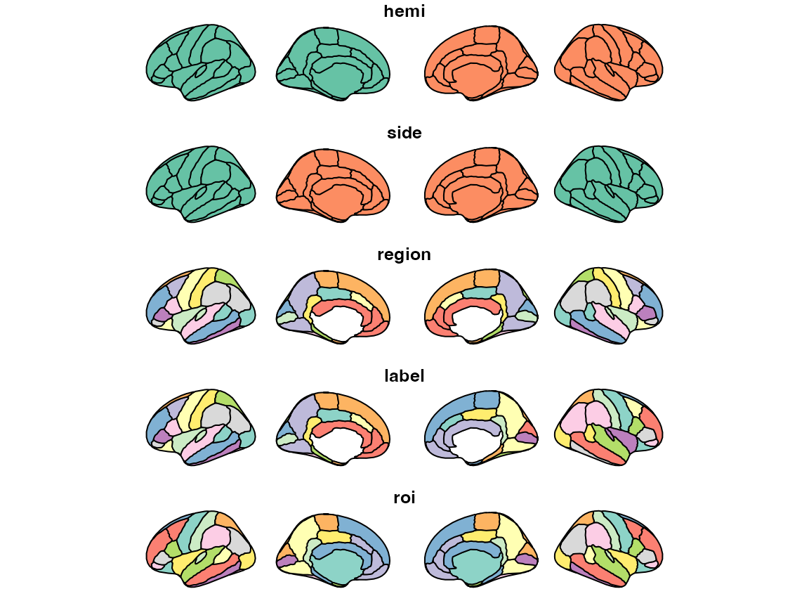
Even better, though, you should call plot directly on
the atlas object. This will give you a fast overview of the atlas you
are thinking of using.
plot(dk)
You will notice that the new atlas-class has better resolution and default values that what you get from the ggseg-atlas class.
Extracting atlas information
This new class also comes with a new custom printout method, that should give you a better idea of the atlas content. It lists information such as:
- type of atlas
- number of unique regions
- hemispheres
- slice views
- whether it has a built-in palette
And in addition it has a preview of the data content, so you may more easily discern how you might adapt your own data to fit the atlas data.
dk
#> # dk cortical brain atlas
#>   regions: 35
#>   hemispheres: left, right
#>   side views: lateral, medial
#>   palette: yes
#>   use: ggplot() + geom_brain()
#> ----
#>    hemi  side    region                label                   roi
#>    <chr> <chr>   <chr>                 <chr>                   <chr>
#>  1 left  lateral bankssts              lh_bankssts             0002
#>  2 left  lateral caudal middle frontal lh_caudalmiddlefrontal  0004
#>  3 left  lateral fusiform              lh_fusiform             0008
#>  4 left  lateral inferior parietal     lh_inferiorparietal     0009
#>  5 left  lateral inferior temporal     lh_inferiortemporal     0010
#>  6 left  lateral lateral occipital     lh_lateraloccipital     0012
#>  7 left  lateral lateral orbitofrontal lh_lateralorbitofrontal 0013
#>  8 left  lateral middle temporal       lh_middletemporal       0016
#>  9 left  lateral pars opercularis      lh_parsopercularis      0019
#> 10 left  lateral pars orbitalis        lh_parsorbitalis        0020
#> # ℹ 76 more rows
Some users have also wanted to easier ways of checking the names of regions and labels of an atlas, in order to check if their data fits the atlas data. In order to make this easier, we have added two new functions that should help you with that.
brain_regions(dk)
#>  [1] "bankssts"                   "caudal anterior cingulate"
#>  [3] "caudal middle frontal"      "corpus callosum"
#>  [5] "cuneus"                     "entorhinal"
#>  [7] "frontal pole"               "fusiform"
#>  [9] "inferior parietal"          "inferior temporal"
#> [11] "insula"                     "isthmus cingulate"
#> [13] "lateral occipital"          "lateral orbitofrontal"
#> [15] "lingual"                    "medial orbitofrontal"
#> [17] "middle temporal"            "paracentral"
#> [19] "parahippocampal"            "pars opercularis"
#> [21] "pars orbitalis"             "pars triangularis"
#> [23] "pericalcarine"              "postcentral"
#> [25] "posterior cingulate"        "precentral"
#> [27] "precuneus"                  "rostral anterior cingulate"
#> [29] "rostral middle frontal"     "superior frontal"
#> [31] "superior parietal"          "superior temporal"
#> [33] "supramarginal"              "temporal pole"
#> [35] "transverse temporal"
brain_labels(dk)
#>  [1] "lh_bankssts"                 "lh_caudalanteriorcingulate"
#>  [3] "lh_caudalmiddlefrontal"      "lh_corpuscallosum"
#>  [5] "lh_cuneus"                   "lh_entorhinal"
#>  [7] "lh_frontalpole"              "lh_fusiform"
#>  [9] "lh_inferiorparietal"         "lh_inferiortemporal"
#> [11] "lh_insula"                   "lh_isthmuscingulate"
#> [13] "lh_lateraloccipital"         "lh_lateralorbitofrontal"
#> [15] "lh_lingual"                  "lh_medialorbitofrontal"
#> [17] "lh_middletemporal"           "lh_paracentral"
#> [19] "lh_parahippocampal"          "lh_parsopercularis"
#> [21] "lh_parsorbitalis"            "lh_parstriangularis"
#> [23] "lh_pericalcarine"            "lh_postcentral"
#> [25] "lh_posteriorcingulate"       "lh_precentral"
#> [27] "lh_precuneus"                "lh_rostralanteriorcingulate"
#> [29] "lh_rostralmiddlefrontal"     "lh_superiorfrontal"
#> [31] "lh_superiorparietal"         "lh_superiortemporal"
#> [33] "lh_supramarginal"            "lh_temporalpole"
#> [35] "lh_transversetemporal"       "rh_bankssts"
#> [37] "rh_caudalanteriorcingulate"  "rh_caudalmiddlefrontal"
#> [39] "rh_corpuscallosum"           "rh_cuneus"
#> [41] "rh_entorhinal"               "rh_frontalpole"
#> [43] "rh_fusiform"                 "rh_inferiorparietal"
#> [45] "rh_inferiortemporal"         "rh_insula"
#> [47] "rh_isthmuscingulate"         "rh_lateraloccipital"
#> [49] "rh_lateralorbitofrontal"     "rh_lingual"
#> [51] "rh_medialorbitofrontal"      "rh_middletemporal"
#> [53] "rh_paracentral"              "rh_parahippocampal"
#> [55] "rh_parsopercularis"          "rh_parsorbitalis"
#> [57] "rh_parstriangularis"         "rh_pericalcarine"
#> [59] "rh_postcentral"              "rh_posteriorcingulate"
#> [61] "rh_precentral"               "rh_precuneus"
#> [63] "rh_rostralanteriorcingulate" "rh_rostralmiddlefrontal"
#> [65] "rh_superiorfrontal"          "rh_superiorparietal"
#> [67] "rh_superiortemporal"         "rh_supramarginal"
#> [69] "rh_temporalpole"             "rh_transversetemporal"
Plotting the atlas
For other than quick overviews of the atlas using plot
this new atlas class is specifically made to work with the new
geom_brain. Since we have better control over the geom, we
have also optimized it so that when plotting just the atlas, without
specifying fill the polygons are automatically filled with
the region column.
ggplot() +
  geom_brain(atlas = dk)
This new geom makes it possible for you to also better control the
position of the brain slices, using specialized function for this to the
position argument. The position_brain function takes a
formula argument similar to that of facet_grid to alter the
positions of the slices.
ggplot() +
  geom_brain(atlas = dk, position = position_brain(hemi ~ side))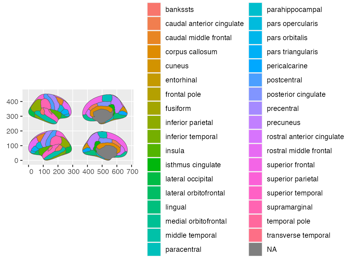
A new addition to the positions, is the ability to also specify the order directly through a character vector. By default, the position is:
cortical_pos <- c(
  "left lateral",
  "left medial",
  "right medial",
  "right lateral"
)
ggplot() +
  geom_brain(atlas = dk, position = position_brain(cortical_pos))
# Which can easily be switched around!
cortical_pos <- c(
  "right lateral",
  "left medial",
  "right medial",
  "left lateral"
)

ggplot() +
  geom_brain(atlas = dk, position = position_brain(cortical_pos))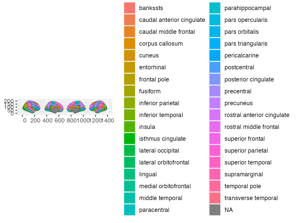
Reducing slices
Many have wanted the option like in ggseg() to only see
a single hemisphere or slice. This functionality had been added through
the hemi and side arguments to
geom_brain(), mimicking the way ggseg()
works.
ggplot() +
  geom_brain(atlas = dk, side = "lateral")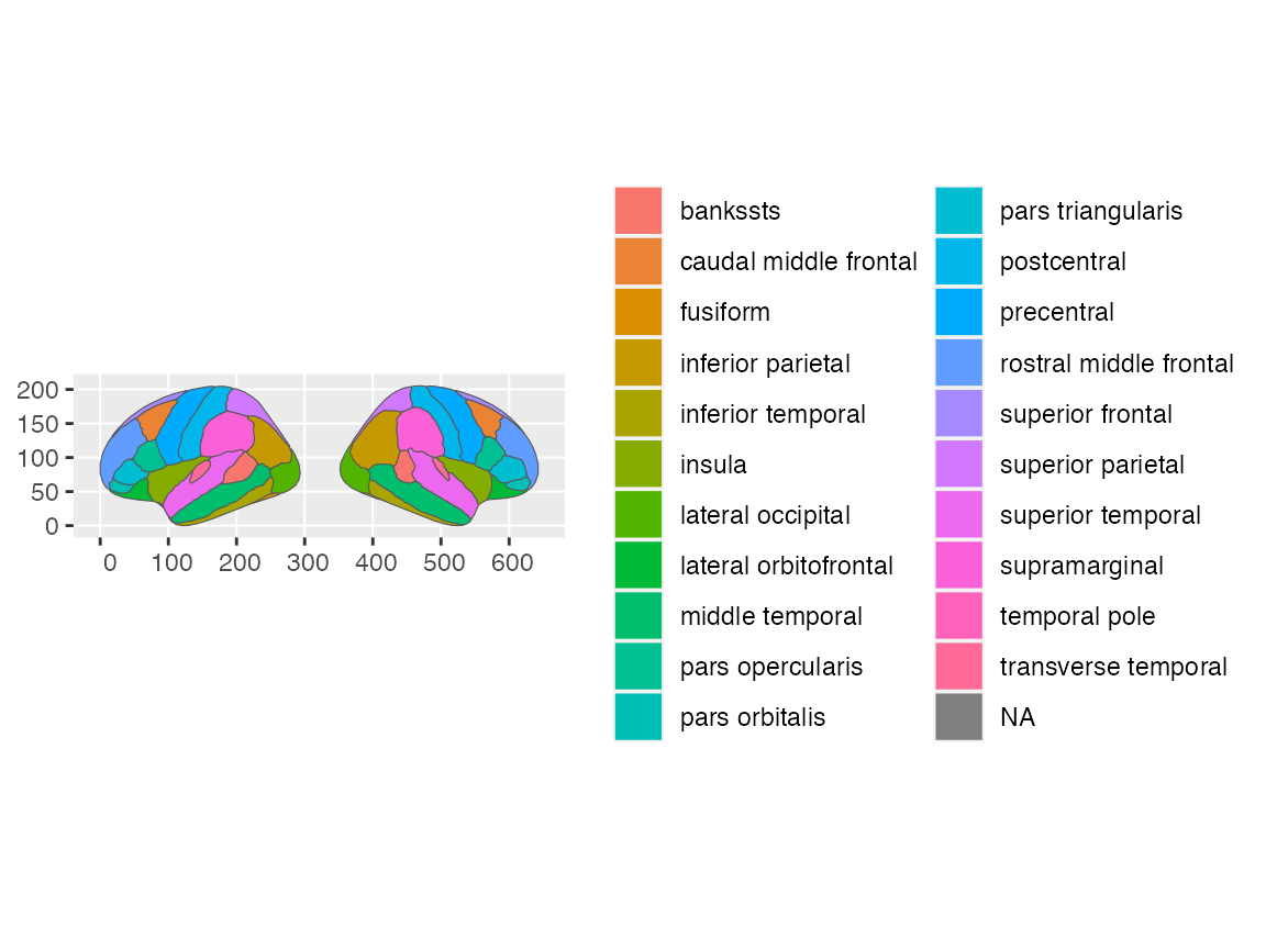
ggplot() +
  geom_brain(atlas = dk, hemi = "left")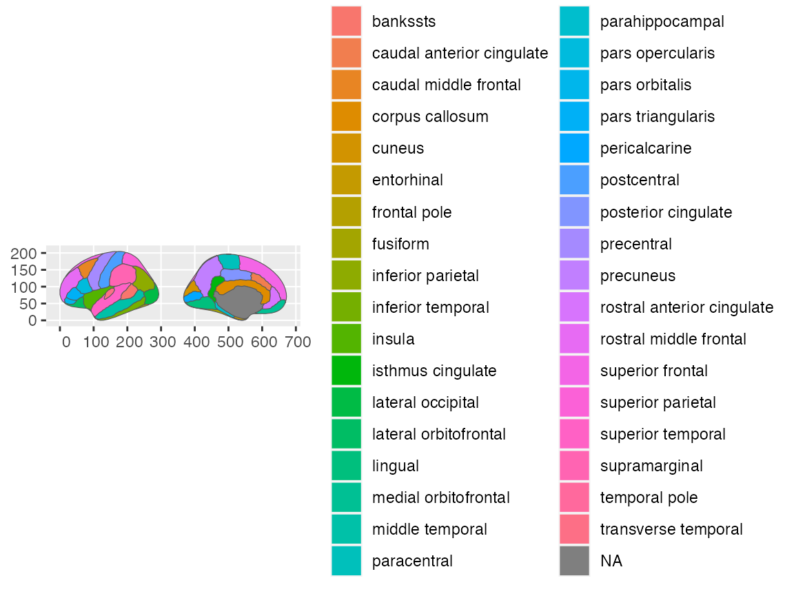
This also should work for subcortical atlases, but the hemisphere
(hemi) specification should be used carefully, as it might
end up looking quite different than what you intended!
ggplot() +
  geom_brain(atlas = aseg, side = "coronal", hemi = "left")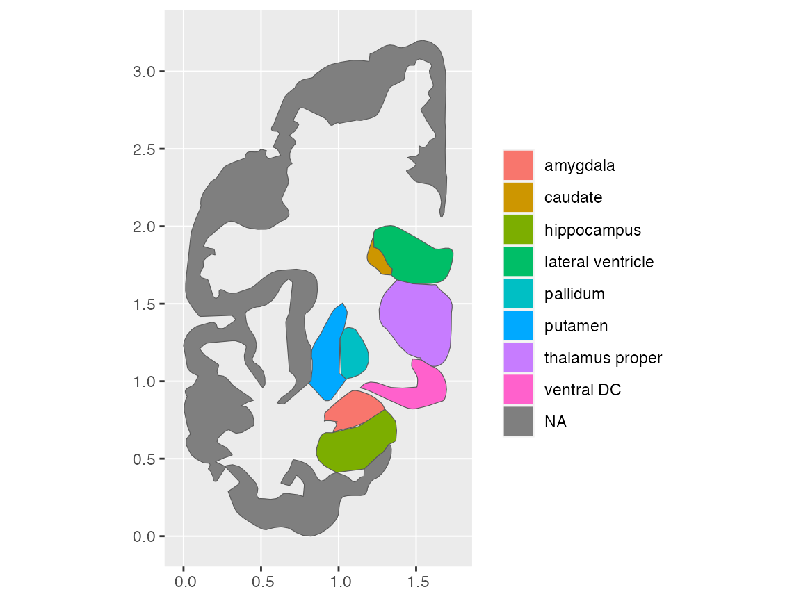
Plotting with data
Of course, as usual, people will have their own data they want to add to the plots, using columns from their own data to the plot aesthetics. By making sure at least one column in your data has the same name and overlapping content as a column in the atlas data, geom_brain will merge your data with the atlas and create your plots.
library(dplyr)
#>
#> Attaching package: 'dplyr'
#> The following objects are masked from 'package:stats':
#>
#>     filter, lag
#> The following objects are masked from 'package:base':
#>
#>     intersect, setdiff, setequal, union

some_data <- tibble(
  region = c(
    "transverse temporal",
    "insula",
    "precentral",
    "superior parietal"
  ),
  p = sample(seq(0, .5, .001), 4)
)

some_data
#> # A tibble: 4 × 2
#>   region                  p
#>   <chr>               <dbl>
#> 1 transverse temporal 0.172
#> 2 insula              0.406
#> 3 precentral          0.459
#> 4 superior parietal   0.062
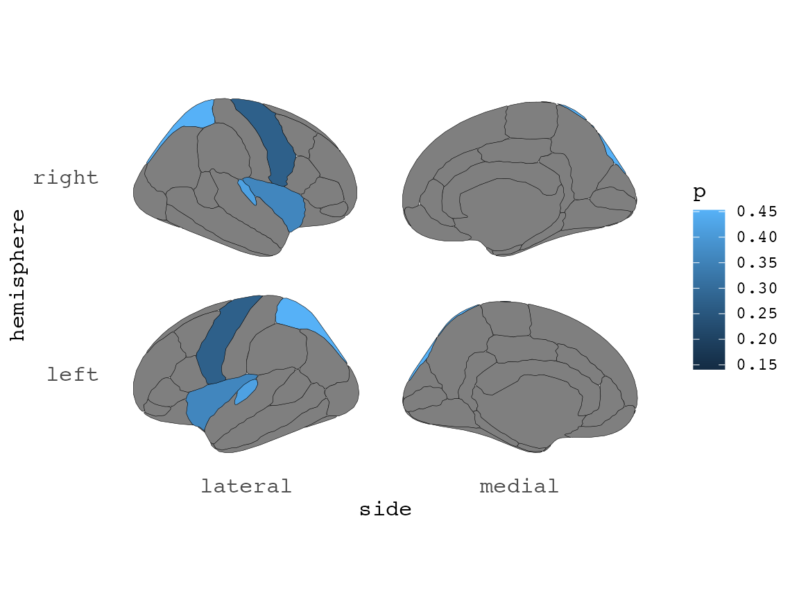
And such plots can be further adapted with standard ggplot themes, scales etc, to your liking.
ggplot(some_data) +
  geom_brain(
    atlas = dk,
    position = position_brain(hemi ~ side),
    aes(fill = p)
  ) +
  scale_fill_viridis_c(option = "cividis", direction = -1) +
  theme_void() +
  labs(
    title = "My awesome title",
    subtitle = "of a brain atlas plot",
    caption = "I'm pretty happy about this!"
  )
#> merging atlas and data by 'region'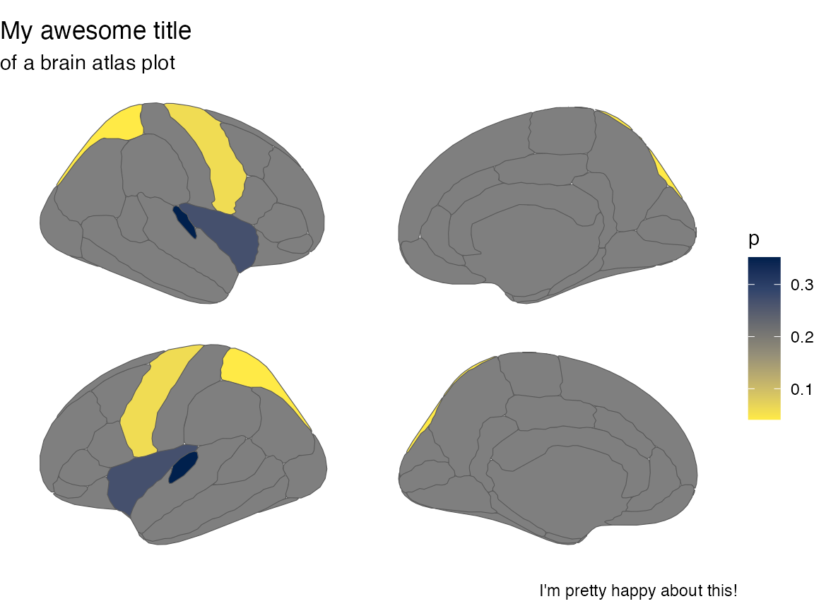
Facet group data
Just like in ggseg, though, you still need to do some double work for
faceting to work correctly. Because the atlas and your data need to be
merged correctly, you will need to group_by your data
before giving it to ggplot, for facets to work.
some_data <- tibble(
  region = rep(
    c(
      "transverse temporal",
      "insula",
      "precentral",
      "superior parietal"
    ),
    2
  ),
  p = sample(seq(0, .5, .001), 8),
  groups = c(rep("g1", 4), rep("g2", 4))
)

some_data
#> # A tibble: 8 × 3
#>   region                  p groups
#>   <chr>               <dbl> <chr>
#> 1 transverse temporal 0.484 g1
#> 2 insula              0.357 g1
#> 3 precentral          0.366 g1
#> 4 superior parietal   0.046 g1
#> 5 transverse temporal 0.414 g2
#> 6 insula              0.451 g2
#> 7 precentral          0.485 g2
#> 8 superior parietal   0.2   g2
some_data |>
  group_by(groups) |>
  ggplot() +
  geom_brain(
    atlas = dk,
    position = position_brain(hemi ~ side),
    aes(fill = p)
  ) +
  facet_wrap(~groups) +
  ggtitle("correct facetting")
#> merging atlas and data by 'region'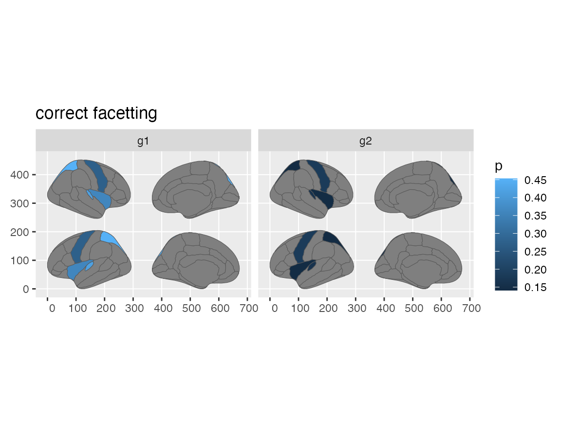
Plotting regions as categorical
You can call plot() on any ggseg-atlas and get a preview
of the entire atlas, with labels for each region.
plot(dk)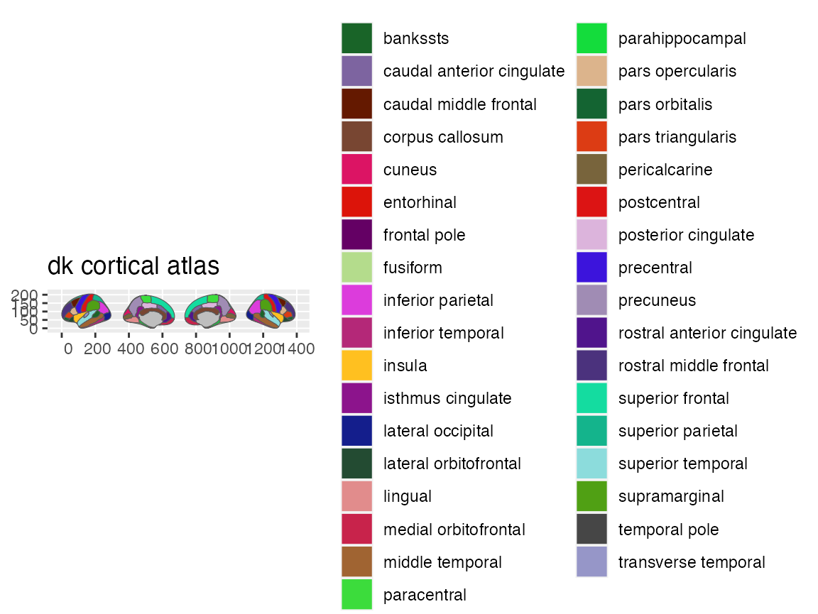
Sometimes, though, you might still want to plot regions as categorical, but only a subset of them. To do this, we need to do a little hack. Since the ggseg plotting function copies over the entire atlas (so it can display each region), we need two columns in the incoming data. One to merge nicely with the atlas data and one to specify which regions to colour. These two columns will likely contain mirrored information, but with different names.
data <- data.frame(
  region = brain_regions(dk)[1:3],
  reg_col = brain_regions(dk)[1:3]
)

data
#>                      region                   reg_col
#> 1                  bankssts                  bankssts
#> 2 caudal anterior cingulate caudal anterior cingulate
#> 3     caudal middle frontal     caudal middle frontal

ggplot(data) +
  geom_brain(atlas = dk, aes(fill = reg_col)) +
  scale_fill_brain2(dk$palette[data$region])
#> merging atlas and data by 'region'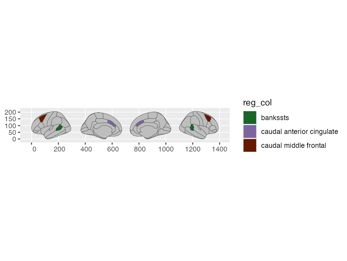
Plotting with ggseg
You can also plot this new atlas class directly with the
ggseg function, if you are more comfortable with that.
ggseg(
  some_data,
  atlas = dk,
  colour = "black",
  size = .1,
  position = "stacked",
  mapping = aes(fill = p)
)
#> merging atlas and data by 'region'
#> Warning: Using `size` aesthetic for lines was deprecated in ggplot2 3.4.0.
#> ℹ Please use `linewidth` instead.
#> ℹ The deprecated feature was likely used in the ggseg package.
#>   Please report the issue at <https://github.com/ggseg/ggseg/issues>.
#> This warning is displayed once every 8 hours.
#> Call `lifecycle::last_lifecycle_warnings()` to see where this warning was
#> generated.