FreeSurfer already have files that are compatible with
ggseg in some extent. There are naming conventions and
file-formats that are different, and as such it can at times be a little
tricky to get data directly from FreeSurfer into R, and subsequently
plotting in ggseg.
Raw stats files
Read in single raw stats file
If recon-all from FreeSurfer has been run, each
participant should have a stats folder, with various
parcellation data and summary statistics for those parcellations and
measures. These have many header lines before the data actually start,
and can have some formatting difficult to handle in R.
The function read_freesurfer_stats is made to easily
read in raw stats tables from each individual, without needing to go
through FreeSurfer’s internal converters. When using this file,
remembering which hemisphere is read in is important, as this
information must be added to the label column for
ggseg to recognize the region labels.
stats_file <- file.path(subjects_dir, "bert/stats/lh.aparc.stats")
data <- read_freesurfer_stats(stats_file)
data
#> # A tibble: 34 × 10
#>    label    NumVert SurfArea GrayVol ThickAvg ThickStd MeanCurv GausCurv FoldInd
#>    <chr>      <int>    <int>   <int>    <dbl>    <dbl>    <dbl>    <dbl>   <int>
#>  1 bankssts    1181      831    2297     2.77    0.428    0.116    0.024      11
#>  2 caudala…     843      572    1534     2.72    0.469    0.124    0.013      10
#>  3 caudalm…    2758     1840    5772     2.80    0.526    0.114    0.021      26
#>  4 cuneus      2683     1654    3074     1.81    0.471    0.14     0.033      39
#>  5 entorhi…     581      416    1840     3.33    0.667    0.116    0.032       5
#>  6 fusiform    4113     2875    8519     2.72    0.599    0.131    0.025      52
#>  7 inferio…    4948     3466   10559     2.70    0.509    0.131    0.029      65
#>  8 inferio…    5056     3542   12358     2.98    0.625    0.138    0.033      74
#>  9 isthmus…    1561      990    2350     2.09    0.745    0.113    0.023      19
#> 10 lateral…    7961     5077   12743     2.30    0.588    0.139    0.033     104
#> # ℹ 24 more rows
#> # ℹ 1 more variable: CurvInd <dbl>
This data should be well-suited for use with ggseg.
library(dplyr)
data |>
  mutate(label = paste0("lh_", label)) |>
  ggseg(atlas = dk, mapping = aes(fill = ThickAvg))
#> merging atlas and data by 'label'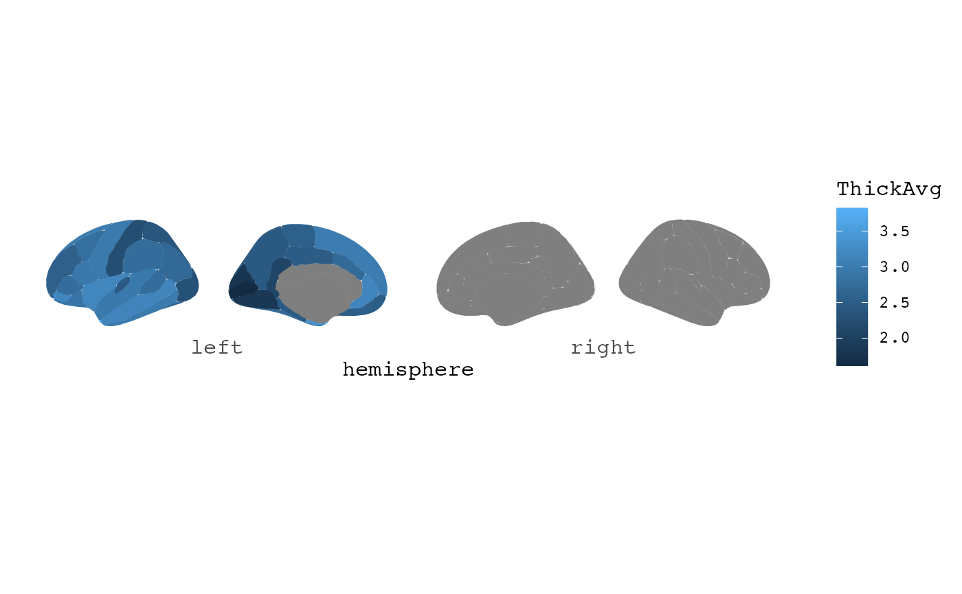
Read in raw stats files for an atlas for all subjects
A convenience function also exists for those wanting to circumvent
the aparcstats2table and asegstats2table from
freesurfer for creating larger datasets of all subjects for a specific
parcellation and metric. Using the function
read_freesurfer_stats, read_atlas_files uses
regular expression for the atlas you want to extract data from, and
grabs this data from all available subjects. Be careful with your
pattern matching to be sure you get exactly the atlas you want. For
instance, there are several atlases with with string aparc
in them. So in order to get only the default aparc stats, we need to
specify aparc.stats$, which will only read those files
ending with that particular string. This function can throw
warnings, which is most cases can be ignored.
dat <- read_atlas_files(subject_dir, "aparc.stats$")
dat
#> # A tibble: 68 × 11
#>    subject label    NumVert SurfArea GrayVol ThickAvg ThickStd MeanCurv GausCurv
#>    <chr>   <chr>      <int>    <int>   <int>    <dbl>    <dbl>    <dbl>    <dbl>
#>  1 bert    lh_bank…    1181      831    2297     2.77    0.428    0.116    0.024
#>  2 bert    lh_caud…     843      572    1534     2.72    0.469    0.124    0.013
#>  3 bert    lh_caud…    2758     1840    5772     2.80    0.526    0.114    0.021
#>  4 bert    lh_cune…    2683     1654    3074     1.81    0.471    0.14     0.033
#>  5 bert    lh_ento…     581      416    1840     3.33    0.667    0.116    0.032
#>  6 bert    lh_fusi…    4113     2875    8519     2.72    0.599    0.131    0.025
#>  7 bert    lh_infe…    4948     3466   10559     2.70    0.509    0.131    0.029
#>  8 bert    lh_infe…    5056     3542   12358     2.98    0.625    0.138    0.033
#>  9 bert    lh_isth…    1561      990    2350     2.09    0.745    0.113    0.023
#> 10 bert    lh_late…    7961     5077   12743     2.30    0.588    0.139    0.033
#> # ℹ 58 more rows
#> # ℹ 2 more variables: FoldInd <int>, CurvInd <dbl>
Since all files are read in, the hemisphere in the label is already fixed, so it is easy to plot.
With this data, we can even have a look at all the metrics at once.
library(dplyr)
library(tidyr)

dat |>
  gather(stat, val, -subject, -label) |>
  group_by(stat) |>
  ggseg(mapping = aes(fill = val)) +
  facet_wrap(~stat)
#> merging atlas and data by 'label'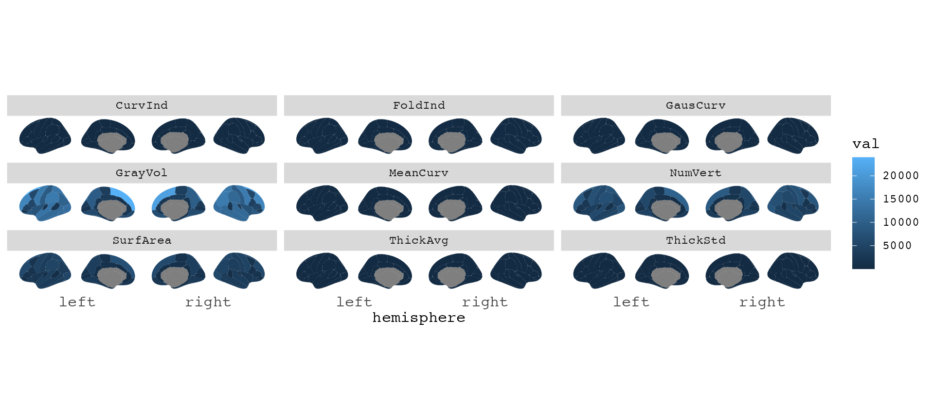
FreeSurfer stats tables
FreeSurfer has internal functions to convert their raw stats files
into tables, gather subject into a single data file with particular
metric. It is quite common to use these files, but again the formatting
is not something R is very happy with. The function
read_freesurfer_table() is for easier import of these
files, particularly for further plotting with ggseg.
# Path to our particular file, yours will be wherever you have saved it
table_path <- here::here("tests/testthat/data/aparc.volume.table")
table_path
#> [1] "/home/runner/work/ggseg/ggseg/tests/testthat/data/aparc.volume.table"
read_freesurfer_table(table_path)
#> # A tibble: 36 × 3
#>    subject label                             value
#>    <chr>   <chr>                             <dbl>
#>  1 bert    rh_bankssts_volume                 1969
#>  2 bert    rh_caudalanteriorcingulate_volume  2280
#>  3 bert    rh_caudalmiddlefrontal_volume      5390
#>  4 bert    rh_cuneus_volume                   2998
#>  5 bert    rh_entorhinal_volume               1735
#>  6 bert    rh_fusiform_volume                 8144
#>  7 bert    rh_inferiorparietal_volume        14876
#>  8 bert    rh_inferiortemporal_volume        11016
#>  9 bert    rh_isthmuscingulate_volume         1983
#> 10 bert    rh_lateraloccipital_volume        12729
#> # ℹ 26 more rows
The file is read and has three columns only. The subject column, the
label column, and a column with the values of the metric. Since the
stats tables can contain different measures, and these are handled
somewhat differently, we for convenience leave the default reading of
the table this way. To work with ggseg, though, the labels usually (but
not always) need a little cleaning. In this case we read in a
volume table, and as such all labels end with “_volume”.
ggseg will not recognize this matching the atlas, and will
therefore not plot.
Easiest way to clean, is by using the measure argument
for the function.
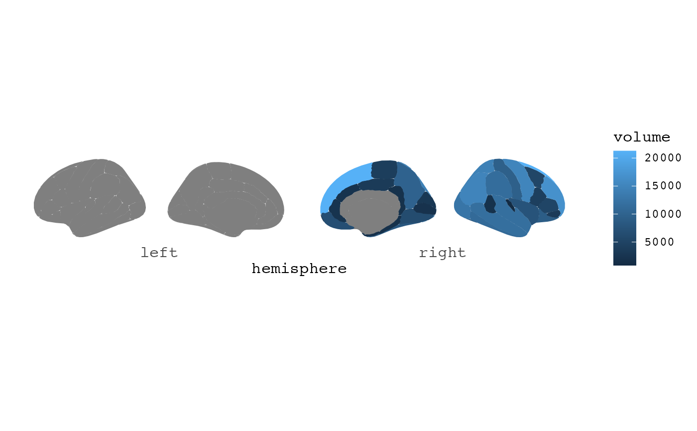
dat <- read_freesurfer_table(table_path, measure = "volume")
dat
#> # A tibble: 36 × 3
#>    subject label                      volume
#>    <chr>   <chr>                       <dbl>
#>  1 bert    rh_bankssts                  1969
#>  2 bert    rh_caudalanteriorcingulate   2280
#>  3 bert    rh_caudalmiddlefrontal       5390
#>  4 bert    rh_cuneus                    2998
#>  5 bert    rh_entorhinal                1735
#>  6 bert    rh_fusiform                  8144
#>  7 bert    rh_inferiorparietal         14876
#>  8 bert    rh_inferiortemporal         11016
#>  9 bert    rh_isthmuscingulate          1983
#> 10 bert    rh_lateraloccipital         12729
#> # ℹ 26 more rows
This will do two things: 1) remove the label suffix, and 2) rename
the value column to the measure supplied. Alternatively,
you will need to do string manipulation on the label column your self,
we recommend the stringr package in
that case.
An error will be thrown because the FreeSurfer tables also include measures of total volume/region/thickness, estimated intracranial volume etc, which will not merge into the atlas, and the internal ggseg atlas-merging function throws a warning. To avoid this, you can remove those labels before plotting.
dat |>
  filter(grepl("lh|rh", label)) |>
  ggseg(mapping = aes(fill = volume))
#> merging atlas and data by 'label'